Procedural Sphere / Ellipsoid Tutorial

DISCLAIMER #1: Code presented here is pseudocode that does NOT necessarily reflect production Limit Theory code.

DISCLAIMER #2: This tutorial assumes you have at least basic knowledge of 3D geometry and related math.

I’ve seen plenty of tutorials for procedural spheres online, but most of them present the pseudocode (or even worse, language-specific code) for a sphere without explaining why it works. But if you want to really learn how to create procedural meshes – especially creative ones like torii or mesh warps like stellation and extrusion – it helps massively to first understand how the simple ones work.

Note: This tutorial specifically focuses on the UV-sphere method of creating a sphere. If you’re interested in the icosahedron-sphere / “icosasphere” method of creating a sphere, stay tuned- I’m creating a tutorial for icosahedrons soon 🙂 And regardless of the method, the learning process you’ll go through while creating a sphere, with any method, will help you understand more about procedural geometry.

To begin, we’ll first look at how to create a sphere, then adapt that algorithm for any general ellipsoid (a sphere-shape with arbitrary width, length, and height).

First, let’s lay out the general equation for all of the verticies in a circle:

for theta = 0, 2*pi
x = cos(theta) * radius
y = sin(theta) * radius

We know this works because this is the parametric equation for a circle. “Parametric” in this context means that the output values, in this case, the cartesian coordiantes [x, y] (or [x, y, z] in 3d), are a function of an angle theta. So essentially, we’re going around in a circle in space and placing a point at every angle between 0 to 2*pi. I recommend clicking the link above for some visuals in case you aren’t grok-ing this from words alone.

Of course, we need to have a discrete (non-infinite) number of points to store for verticies. Notice, if you wanted to, you could either have a very small number of points to create regular polygons, like octagons, or a very high number of points to give the illusion of roundness. We’re going for the latter for this tutorial. Given “n” to describe the number of subdivisions of the circle, our equation now looks like this:

verticies = {}
dt = (2*pi)/n
for t = 0, 2*pi, dt
  v = Vec2()
  v.x = cos(t) * radius
  v.y = sin(t) * radius
  verticies.add(v)
end

Now that we understand how the algorithm for a circle with an arbitrary number of subdivisions works, we’re ready to bring this into 3D!

In 3D, we now need two loops: an inner loop to draw every 2D circle of verticies (which are made up of slices, as in the vertical lines shown on the left sphere below), and an outer loop to stack those rings and give them a varying radius (which I’m calling stacks, as in the horizontal lines on the sphere).

(and a sassy cat to make fun of my freehanded circles.)

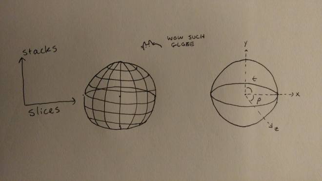
We vary the radius of each stack by making the radius a function of its y-position. As you can see, the radius of each stack is the largest at the center and tapers off towards the top and bottom of the sphere. This algorithm gives the vertical radius by stackRadius and then calculates every vertex in each slice using the

n = 25 -- arbitrary # of subdivisions
radius = 1 -- arbitrary radius

local theta = pi/n   -- see "t" above
local phi = (2*pi)/n -- see "p" above

verticies = {}
for stack = 0, n - 1 do
  stackRadius = sin(theta * stack) * radius
  for slice = 0, n - 1 do
    x = cos(phi * slice) * stackRadius
    y = cos(theta * stack) * radius
    z = sin(phi * slice) * stackRadius
    verticies.add(x, y, z)
  end
end

n = 25 -- arbitrary # of subdivisions
radius = 1 -- arbitrary radius

local theta = pi/n -- see "t" above
local phi = (2*pi)/n -- see "p" above

verticies = {}
verticies.add(0, radius, 0) -- top vertex
for stack = 1, n - 1 do
  stackRadius = sin(theta * stack) * radius
  for slice = 0, n - 1 do
    x = cos(phi * slice) * stackRadius
    y = cos(theta * stack) * radius
    z = sin(phi * slice) * stackRadius
    verticies.add(x, y, z)
  end
end
verticies.add(0, radius, 0) -- bottom vertex

n = 25 -- arbitrary # of subdivisions
radius = 1 -- arbitrary radius

local theta = pi/n
local phi = (2*pi)/n

verticies = {}
verticies.add(0, radius, 0)
for stack = 1, n - 1 do
  stackRadiusX = sin(theta * stack) * width
  stackRadiusZ = sin(theta * stack) * length
  for slice = 0, n - 1 do
    x = math.cos(phi * slice) * stackRadiusX
    y = math.cos(theta * stack) * height
    z = math.sin(phi * slice) * stackRadiusZ
    verticies:add(x, y, z)
  end
end
verticies.add(0, radius, 0)

• Try drawing it out for yourself and see if you can match it with the algorithm presented below. Reference the hand-drawn picture of a globe above, and how it’s split into quads. (Remember that a quad is just two tris!)
• In the pseudocode below, each vertical column of quads is called a “slice”, and each horizontal row is called a “stack”. We traverse the ellipsoid from bottom to top, visiting each slice on every vertical stack.
• Notice that when we finish a slice and we’re building the last quad on each row, we need to loop the indicies back around to the first index for that row.

tris = {}

-- top tris
for slice = 0, n - 2 do
  -- 0 is the index of the top center point
  tris.add(0, slice +2, slice +1)
end
tris.add(0, 1, res)

-- side quads
for stack = 0, res - 3 do
  for slice = 0, res - 2 do
    local i1 = 1 + slice + (res * stack)
    local i2 = i1 +1
    local i3 = 1 + slice + (res * (stack+1))
    local i4 = i3 + 1
    tris.add(i1, i2, i4)
    tris.add(i1, i4, i3)
  end
  -- last quad on each row
  local i1 = res * (stack +1)
  local i2 = 1 + (res * stack)
  local i3 = res * (stack +2)
  local i4 = 1 + (res * (stack+1))
  tris.add(i1, i2, i4)
  tris.add(i1, i4, i3)
end

-- bottom tris
local lvi = self:getVertexCount() - 1
for slice = 0, res - 2 do
  local i2 = (res-2)*res + slice +1
  local i3 = (res-2)*res + slice +2
  -- lvi is the index of the bottom center point
  tris.add(lvi, i2, i3)
end
tris.add(lvi, (res-1)*res, (res-2)*res +1)

 

If you enjoyed this tutorial, see any typos or bugs, or have any other feedback, leave me a comment or tweet at me! You can follow me here on WordPress or on Twitter @so_good_lin. And be sure to keep track of @LimitTheory on Twitter  – when it comes out, the production version of all of this code & more will be available for exploring and modding. 🙂

DISCLAIMER: Code presented here is pseudocode that does NOT necessarily reflect production Limit Theory code.